Regression Modeling Strategies: Multivariable Modeling Strategies
This is the fourth of several connected topics organized around chapters in Regression Modeling Strategies. The purposes of these topics are to introduce key concepts in the chapter and to provide a place for questions, answers, and discussion around the chapter’s topics.
Additional Links
RMS4
Q&A From May 2021 Course
- It seems like being able to really understand degrees of freedom is important to the overall approach proposed by Frank. I’ve looked over BBR notes but still don’t feel really confident in saying what ‘counts’ as a DF or not. Anywhere you can point us for more information? In particular, if you are, say, making a model to estimate an effect from observational data and you adjust for confounders, does that use up degrees of freedom, or does that not matter because we aren’t actually interested in what the β coefficients are for those confounders? FH: The BBR description is the best one I have right now. Would be interested in getting suggestions for other angles to try. Thanks a lot - what about the question regarding confounders? FH: In many cases the need to adequately control for confounding outweighs considerations about overall model predictive accuracy, so we adjust for more variables than we would normally include in the model and let the width of the confidence interval for the exposure variable effect get a little wide as a result.
- Why is it so important to be masked to the form of the variable when modelling? I was confused by what the plot(anova(f)) was showing - is it a measure of the importance of the variables that are then used to decide which variables to include in the model? This sort of ‘feels’ like using p-values from univariate associations to select predictors but I assume I am missing something. FH: It is not using anything to select predictors. It assumes predictors are already selected. DGL: It is important in variable selection in model development to shield yourself from ‘peaking’ at the form of the relationships between X’s and Y to avoid spurious overfitting and to preserve the alpha error (think big picture/long term). Otherwise there are phantom df’s used that make your SE’s too good and your p-values too small, because you are not honestly ‘pre-’specifying a model. You can make some constrained decisions about where to spend your df’s (allocate information to capture complexity) but because you are not directly using information from Y about the functional form of the relationship, it helps to mitigate the better part of the overfitting. Imagine (as actually happens) nearly everyone over-optimizing the fit for the data they have and getting (and publishing) the smallest p-values, only to find (without penalty) that the predictive capacity does not hold up in future observations. Just imagine!! Does that help? Think ‘big picture’.
- I have two questions regarding the plot(anova(f)). Let’s say we have 20 d.f. to spend and we fit a full model with e.g: 5 binary variables (there goes 5 d.f.), and 5 continuous variables with 4 knots each, (there goes 15 d.f. Which adds up a total of 20 d.f.). Our model is saturated. We now perform the plot(anova(f)) and we see that 3 of the 5 continuous variables have the highest chi2-df value, while 2 cont. var. have a very low chi2-df value. According to the notes, we can change the number of knots in these 2 variables to 0 (hence treating it linearly). Here comes my first question: the anova plot tells us that the predictive “punch” of the continuous variable for Outcome Y is not strong, and therefore we take out the knots and force linearity, but couldn’t it be that the variable is indeed non-linear? We would still be doing an error considering it linear (predictor complexity figure). My best educated guess would be that because the variable is not a good predictor, this error will not affect our predictions that much, hence we can take out the knots without major problems… but I don’t know. My second question is: if we remove the 3 knots (and put 0 knots) to the 2 continous variables that had a very low chi2-df number, we have now gain 2 extra d.f. Could we give these 2 d.f. to the continous variables with the highest chi2-df value, by giving 2 more knots (5 knots instead of 3) as we want to model the variable as good as possible? Sorry for the long answer. Thanks in advance! (pedro). FH: You are right the variable being forced to be linear may have all of its effect being nonlinear. The consequence of this error will be small though. Yes you could re-allocate the d.f. As you said.
- Often people report both adjusted and naïve estimates when estimating the effect of an exposure variable. Do you see any value in that? FH: None whatsoever. Adds nothing but confusion and makes some readers doubt the adjusted estimate. DGL: The practice reflects misplaced or misattributed uncertainty. There is no good rationale for eschewing the adjusted in favor of the unadjusted estimate, unless your adjustment is really wholly arbitrary (and therefore pointless).
- I’ve never done simulations before and I am confused how it applies to variable selection. I am a student, and this is the first time I’m hearing about this. Can you give the step-by-step on how to go about simulations? For example, let’s say you have a dataset with 1 response and 10 independent variables, Do we first run a regression with 10 independent variables, not prespecified in the model. Then use those coefficients to run a simulation and see if the model is good? How do you then determine which of those 10 are good? How did you generate the coefficients in the simulation in the true model? FH: Start with the code in the simulation we studied today. Modifying it for different sample sizes, true regression coefficients, and number of predictors. Over time you’ll get comfortable with simulation of more complex data analysis procedures including multi-step procedures. DGL Simulation is for developing acumen with your instrument (modeling)—getting intimately facile with it. Like a good swordsman, you want to be comfortable and confident with the tool you are counting on… You should know how to use your tool. Simulation demonstrates for you both how structure (plus some known stochastic error) generates data, and how [known] data manifests in the structure and performance of the model. Simulation gives you a sense of the tolerances of the analysis process. It is a positive (and negative) control. It is a little exercise in ‘divination’: you create the underlying reality and then you see how well the known artificial signal is carried in the process of analysis with MVM. Your intuitions and mastery improve and you become a better judge of things with you only receive data and have to divine the structure and signals latent within.
- Can the R package pmsampsize by Riley et al. for estimating a sample size for a prediction model also be used to adjust for covariates using logistic regression? FH: See a comment above about confounder adjustment. Sample size for achieving predictive accuracy is different (and usually larger than) the sample size needed to have power or prediction for an adjusted exposure effect.
- Sample size needed → pmsampsize in R and Stata. Paper published in BMJ https://www.bmj.com/content/bmj/368/bmj.m441.full.pdf
Regarding Cox Snell R2 (which is needed for the pmsampsize) please see this recent paper A note on estimating the Cox-Snell R 2 from a reported C statistic (AUROC) to inform sample size calculations for developing a prediction model with a binary outcome - PubMed
- Can coefficients after shrinkage be interpreted the same way as coefficients after “normal” regression? FH: Yes DGL: They can be interpreted, moreover, as likely to be more reliable and reproducible in the future—in the long run.
- In addition to shrinkage, there is an issue in the creation of regression models (transfer functions) for paleoclimate reconstruction that requires ‘deshrinkage.’ When reconstructing ancient climate variables like lake or ocean temperature or pH using proxy data like diatom frustules, the initial regression models produce results that are insufficiently variable and with low estimates being too high and high estimates being too low. Ter Braak, Juggins & Birks developed deshrinking methods for their paleoclimate regressions (implemented in Juggins’ R package rioja) to deshrink the regression output improving the fit to the training data This is particularly important in predicting both low and high values of something like pH in ancient climates. I don’t think I’ve ever seen ‘deshrinkage’ used outside of this narrow area of regression modeling. I mentioned this once to Morris after a talk he gave on shrinkage, and he said that it was ridiculous to deshrink regressions. Juggins’ rioja vignette cites the key paper describing deshrinking: https://cran.r-project.org/web/packages/rioja/rioja.pdf FH: I’ve never heard of deshrinking, and my initial reaction is the same as Morris. DGL IMHO—it appeals to me in this particular context, but Bayesean approaches incorporating beliefs and uncertainties might be even better in this epistemologic application, I imagine. But FH would have more insight than I.
- Is there any difference between using ns() and Hmisc::rcspline.eval in fitting a spline model? FH: See the gTrans vignette we covered Wednesday morning. Coefficients are different but predicted values are the same if you use the same knot locations. You have to be explicit about outer knots for ns.
- So far the course focused mainly on models where outcome variables are well defined. I am working on a project of developing a phenotyping algorithm (essentially a prediction model where the predicted probability leads to the phenotype classification) of an underdiagnosed disease using electronic health records on millions of veterans. We plan to develop the algorithm in a semi-supervised framework, and a chart review will be conducted to create golden standard labels on the selected sample. My question is what is the standard for selecting patients for chart review to minimize biases and improve model’s discriminative performance? Is having positive labels (disease = yes) as important as having a negative label? Does the same filter that we apply to select chart review patients should also be applied to the data we can use for final algorithm development (for example, during chart review, we sample patients from those who have either some ICD diagnosis codes or some NLP mentions in clinical notes. When running the final model, does it mean that we should also use data on veterans who passed the same filter to avoid extrapolation.) Thanks! FH: A perfect question for datamethod.org. There are probably some good design papers. I recommend something like a random sample of 200 controls and 200 cases and developing a logistic regression model for P(true positive diagnosis). This will teach you which types of patients can be put in a near-rule-in and near-rule-out category and which ones you should not attempt to diagnose (e.g. probability [0.15, 0.85]).
- Do you ever encounter a situation where a single variable such as age overwhelms all other predictor variables in a model? If so is there any solution? FH: Yes we almost see that in our diabetes case study. The solution is to let age dominate, and give age the flexibility to dominate even more. There are many published prognostic models where the final result was dumbed down to 4 risk categories, but continuous age is a better predictor than the authors’ entire model.
- When using 3-5 level ordinal predictors, do you always recommend creating dummy variables? FH: No, that usually spends too many d.f. Sometimes we use a quadratic. Bayesian modeling provides an elegant way to handle ordinal predictors which is built into the R brms package brm function. Following up on this, does the brms (or rms) package easily allow for changing the reference group for ordinal predictors?
- Where can I find a practical example of the “degree of freedom” approach or just a broader explanation? I get the sense but …practically? Look at BBR.
- I just read a paper (https://www.sciencedirect.com/science/article/abs/pii/S1551741121001613) talking about moderation (interaction) analysis with a binary outcome, where they recommend evaluating interactions both on an additive and multiplicative scales then interpreting their findings. How is this concept relevant to discussions in this course, particularly around the idea of prespecification? Interactions are always present on the additive scale, so they are boring.
- Data reduction Q :I have a dataset of Ankylosing Spondylitis patients and the response is ASAS20 https://eprovide.mapi-trust.org/instruments/assessment-in-ankylosing-spondylitis-response-criteria.
We have baseline variables, age, sex etc. but we also have 88 other variables relating to patient joints for example swollen elbow, tender elbow etc. The data will not support all these variables and so variable reduction would be useful. What method would you advocate for the 88 joint variables? The 88 are all binary (yes/no). Thank you. Eamonn
Look at correspondence analysis for starters.
- Are there methods to combine lasso/elastic net penalties with splines? (why/why not) would this be a good idea? There are some methods; I haven’t read the papers carefully. There is a difficult scaling issue for nonlinear terms.
- Are automated variable selection methods justified if the only goal is to identify the strongest predictors? No
- Would you discuss/compare concepts of Simpson’s paradox/confounding with non-collapsibility of OR/HR? Look at the ANCOVA chapter in BBR.
- A Principal Investigator is interested in heart ejection fraction (EF) and the relationship with a biomarker B-type natriuretic peptide (BNP). They are wanting to categorise EF% in many ways <55% v >55%, <60% v 60% and also multiple categories and do separate analyses in the subgroups; just three of many they are requesting. Is there a convincing argument/reference that can be used to convince them that all these are troublesome and should be replaced by a flexible single analysis of the continuous percentage? Start with showing outcome heterogeneity within one of their intervals especially on the low LVEF side.
- As GWAS sample sizes keep growing do you see any value in employing ridge/lasso/elastic net penalties and consider SNPs jointly, vs the current approach (a series of separate OLS regressions)? Look at horseshoe priors with Bayesian modeling.
- What would you recommend to use instead of AUC, and why? (sorry if I missed this during the lectures) See the blog article Statistically Efficient Ways to Quantify Added Predictive Value of New Measurements | Statistical Thinking
- In survey data, where we need to account for probability weight and survey design features, and we cannot use rms package and plot(anova(f)), what would be another way to check whether a continuous variable should have 5 knots or 2 knots without seeing the p-value from the anova? A few of the rms fitting functions allow weights. But I don’t recommend that weights be used if there are covariates describing the weighting are included in the model. Weights inflate variances and do not condition on known covariates. ? Thanks for your response. I heard what you explained to Andrew. In our projects, we are interested in population estimates and, in addition, we want to consider the design features of clusters and strata to have corrected standard errors. So, I would like to have a way to “mimic” what plot(anova(f)) does.
- Has anyone ever investigated if variable selection is associated with expertise/knowledge of the researcher? I guess it is a function of the knowledge on a specific field and just another heuristic to save cognitive energies! If you mean has someone investigated whether statistical variable selection agrees with experts’ selections, that has been studied enough to know that statistical variable selection is not as reliable.
 I meant if people use variable selection more when they’re not expert or they are new in the field.
- We talked about avoiding using variable selection and instead using data reduction or saturated model or ridge regression. However, in clinical setting there are situation where one has a number of candidate predictors (e.g. 50) and collecting all of them would mean more cost in time/money, so one would be interested in selecting a subset of these predictors not for the purpose of saving df (assuming we have large N), but for practical matters. What is your opinion about variable selection in this setting? In that setting you would have already narrowed down the list so statistical variable selection would no longer be needed. Or I missed something. ? Thanks for your response. To clarify, the 50 initial candidate variables were selected for clinical reasons, but clinicians cannot afford to ask all 50 of them, so they need to have a reduced set of variables (e.g. 15-20) and need statistical variable selection for this purpose.
- Could you elaborate on what phantom d.f. is in the modeling process? The d.f. you think you’ve gotten rid but that are lurking in the background in the form of model uncertainty. In other words, variables that had a chance to be in the model but used Y to find out you didn’t apparently need them. Having phantom d.f. makes SEs be underestimated.
-
Re: interactions. If we have predictors A and B interacted with spline1 and spline2 but no interaction between A and B, and the chunk test shows the interactions with predictor A significant, but the interaction with predictor B not significant, can we remove predictor B and keep predictor A with the splines interactions?
- ? In some cases, the purpose of the study is not to estimate causal effect for a primary predictor with the outcome, and researchers want to explore the association between some variables (not pre-defined) with the outcome. Researchers will usually provide a long list of variables of interest for univariate screening and then do model selection, both of which now I learned that should be avoided. I was wondering for this kind of study, if we should suggest researchers to pre-define the list of variables they want to put in the model based on the max df we can have and do data reduction if needed later? Is there any information we can provide to help researchers to make the decision about the initial variable list? Thank you!
Hi Prof Harell,
I had not attended your course (really wish I could attend one in the future), and I hope it is okay for me to post a question here.
I refer to the section 4.12 of RMS book, the different models:
- Developing Predictive Models
- Developing Models for Effect Estimation
- Developing Models for Hypothesis Testing
I noted from various posts in datamethods [1][2] that univariable analysis is not useful and using it to pre-screen variables for inclusion in the multivariable analysis is not appropriate.
My questions are:
- Should this practice be avoided for all 3 types of models? Or can it be applied for some?
- In the question posted here [1], I understand that the variables are solely chosen due to significant p-values (in which the cut-off of 0.30 is arbitrary). If say, we generate table 1 or univariable analysis, to give some idea of what should be included or excluded, and in the multivariable, we include all statistically significant ones as well as others that are considered clinically important (either through previous studies, or clinical practice) - would this be okay?
Additionally, how are the different models defined in the book? I read Shmueli, G. (2010). To explain or to predict? Statistical Science, 25, 289–310, but I wonder if there’s any distinction in the definition of these. In summary:
- Explanatory modelling:
*Used for testing causal hypotheses – implicates cause and effect
*Here, it is important to identify the roles of each variable on the specific causal pathway for the study question (confounder, collider, mediator or effect modifiers).
- Predictive modelling:
*Used for the purpose of predicting new or future observations. The goal is to predict
the output value (Y) for new observations given their input values (X).
- Descriptive modelling:
*Used for summarizing or representing the data structure in a compact manner (or parsimoniously).
*In other words, it is used for capturing the association between the dependent and independent variables rather than for causal inference or for prediction.
I hope to learn more from you. Thanks!
Regards,
Hanis
Welcome to the site Hanis. Anyone interested in regression modeling strategies is welcome to post on any of the RMS-related topics on datamethods.
Your questions are excellent. First, univariable screening is a bad idea in almost every context. It may do even more damage for explanatory modeling but it fails for all goals. One of the many problems wrong with it is the use of arbitrary thresholds on a nearly irrelevant scale. Using a higher p-value threshold doesn’t make univariable screening a good idea. If you really wanted to achieve some parsimony, @Ewout_Steyerberg has shown that using backwards stepdown variable selection with \alpha=0.5 (yes that’s 0.5 not 0.05) doesn’t do much harm. Such backwards stepdown is done on a full pre-specified model.
Models should be pre-specified to the extent possible, and statistical significance avoided when considering the inclusion of a variable. One example of why this is the case is that a bunch of “insignificant” predictors can explain confounding.
Shmueli has things laid out nicely.
2 Likes
What is “easy” way to present and explain principal components regression analysis to clinicians who don’t understand PCA? Is it the anova table (anova(fit)) or summary(fit) or ggplot(Predict)? Is it possible to do a partial effects plot for principal components and sparse principal components?
Are there good visual graphs to present PCA regression that can show splines?
Regarding degrees of freedom, particularly in the context of random and mixed effects models, see the Introduction of Julian Faraway’s notes on the revision of his book Extending the Linear Model.
The inventor of PCA, Karl Pearson, was well educated in mathematical physics and borrowed the ideas of principal components analysis from rigid body dynamics. Basically a PCA is a rotation of the n-dimensional coordinate system formed by the n explanatory variables. The rotation is done so that the new coordinates correspond to the principal axes of an n-dimensional ellipsoid defined by the variance-covariance matrix. The first principal component corresponds to the long axis of this ellipsoid, the second PC to the second longest axis of the ellipsoid, etc. Put another way, the first PC is a coordinate along the line of maximum variance of the n-dimensional data, the next PC is orthogonal to it and along the line of second largest variance, and so on.
Then PC regression is just a linear regression modeling using the new variables (the PCs) instead of the original variables.
I elaborate on the historical connections with classical physics in this article (PDF) Letter to the Editor: Euler's contribution to mathematics useful in statistics, by H.A. David | Christopher Tong - Academia.edu
2 Likes
In terms of decoding the PC s for a non-statistical audience these are the tricks I would use:
- The list of correlation coefficients for all component predictors against each PC
- For each PC run a forwards stepwise regression to predict the PC from a smaller subset of the component variables. If by luck you can predict PC_1 with R^{2}=0.93 using only 5 predictors out of 15 component variables, you can conclude the PC_1 is dominated by these 5 variables.
- Similarly run recursive partitioning to predict PC_i from the components as an interpretation tool.
- Try battery reduction
Usually better than these is to use sparse PC s so that each PC_i will have many fewer nonzero variable loadings. This effectively combines variable clustering with PCA.
What is the difference between stepwise regression and fast backward step down variable selection?
“Stepwise” includes forward selection, backward stepdown, and all-possible models. Fast backward stepdown refers to making an approximation to full backwards stepdown, such that the sub-models are not really fit but regression coefficients after removing variables are approximated using a multivariate normality assumption.
Stepwise selection you have mentioned is not a good method.
Since Fast backward stepdown is “stepwise”, does that make it a poor method as well?
When is fastbw() appropriate to use? Can that be a way to reduce overfitting?
For fastbw(), does that use AIC to select the best model?
Correct, fast backward stepdown is just as problematic as the others. Use of any of these methods does not reduce overfitting. Neither does using AIC which just amounts to using a different p-value cutoff. The only time I use backwards stepdown (fast or not) is when I am forced to have a smaller model and the number of variables deleted is small.
Used “RMS” package to fit an OLS Reg. The model looks like this: sqrt(Y) ~ rcs(X1, 3) + rcs(X2, 3) + X3.
Coef for X1 is + and for X1’ -. Both sig diff from 0 (print() output).
Both linear and nonlinear effects of X1 were sig (anova() output).
Y and X1 have an inverted U-shaped relationship (ggplot() output).
-
How do I interpret these 3 outputs jointly? In other words, how do I apply the outputs from print() and anova() to the curve I see on the ggplot() output?
-
How do I determine the location of the knot in X1? I suppose this will give me the value of X1 where the inverted U-shaped curve changes its slope? I think the function ‘specs()’ from RMS answers my question, correct? Because I did not specify the location of the 3 knots, does that mean the model chooses their “best” locations? In other words, could there be better positions for them? My main goal here is to determine the position of the middle knot. Ideally would want to estimate this value (point estimate with confidence limits - but maybe too laborious?).
Thanks!
Chapter 2 of the RMS course notes has the background information needed. Interpretation (and especially “significance” testing) of individual coefficients is not relevant for spline functions. Use the multiple degree of freedom “chunk” tests from anova, which bring evidence for association (non-flatness of spline functions).
When you don’t have subject matter knowledge to allow pre-specification of knot locations, the rcs function places knots where the local sample size supports estimation of parameters. This is done by computing quantiles of the predictor. You’ll see in Chapter 2 the table of default quantiles used. specs shows you the knot locations used. The chapter also contains graphs showing exactly what is going on. A knot is where the jolt (also called jerk in physics; this is the 3rd derivative of the function) is allowed to suddenly change. Loosely speaking this is where shape changes are allowed.
We don’t make knots free parameters then try to find the best fitting knots because (1) that would make inference/confidence limits very complex and (2) with restricted cubic splines the location isn’t that important anyway. The number of knots is more important.
1 Like
Ok. So the coeffs I get from ‘print(fit)’ are irrelevant. Perhaps the only relevant info I get from this output is the sig of the LR test and the adj R2, correct?
“Multiple degree of freedom chunk tests from anova”: Is this the output from ‘anova(fit, X)’?
When I put 3 knots at the .10, .5, and .90 quantiles, there is evidence of a non-linear relationship. But when I change the position of the middle knot to other quantiles, the result does not change. What does that mean? What is the point of showing a non-linear (inverted U-shaped) association between X and Y if I can´t show where the curve changes its slope?
From a practical standpoint, this is the most relevant info to be extracted from my model (in my view). I want to show not only that X and Y are associated, but also that their association reverses depending on the value of X. Of note, X is a measure of disease severity (ranging from 5 to 66 in my sample; scale ranges from 0 to 66) and Y is a continuous measure of brain activity.
Could I use linear splines instead? I would pre-specify 3 models (M1,2,3) with 1 knot each, and change the position of the knot for each model (e.g., M1 with the knot at the 4th quantile of X, M2 with the knot at the 5th quantile, and M3 with the knot at the 6th quantile). Then I could compare the 3 models for their fit, or check in which model the non-linear association is sig. Would that be a good approach?
Thank you!
From print individual coefficients and SEs are valuable if a predictor is linear or binary. Overall measures such as the ones you named are always valuable.
Yes anova(fit) gives you most of the chunk tests you need. It also makes it easy to get other ones
As I said previously changing knots doesn’t change things very much if the number of knots stays the same. The “what is the point” question does not make sense. It always helps to graph the whole curve. The fitted curve and its confidence band shows you what you’re seeking.
Linear splines are not very realistic, with their discontinuous first derivatives.
You’re making all this harder than it really is.
2 Likes
Thank you, I appreciate your feedback.
In ‘summary(f)’, is there a way to compute (and then plot) the point estimates and CIs for different effects of the same predictor at once? For example, to compute the point estimates and CIs for the effects of changing X from one quantile to another (.05 up to .95) in a pairwise fashion? The ideia is to have all these effects on the same ‘summary(f)’ output and then display them all on a single ‘plot(summary(f))’. I tried the code below but it did not work:
summary(f, X = c(first, second quantile), X = c(second, third quantile), etc, est.all = FALSE)
I know I could do it one by one, but maybe there’s a better way?
Thanks
This is done with contrast. Type ?contrast.rms for help which includes a ggplot2 example.
1 Like
Thank you.
I had a look at ?contrast.rms but could not figure it out.
Not sure whether I expressed myself well in my last message.
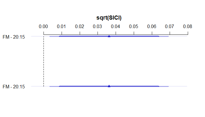
I’m using this code and this is what I’m getting from plot(summary(f)):
s1<-summary(fit2, FM=c(10,15), FM=c(15,20), est.all=FALSE)
plot(s1)
The plot is displaying the effect of changing FM from 15 to 20 twice, instead of also displaying the effect of changing FM from 10 to 15. Do you know why? Is this still a contrast issue?
No, please read my message more carefully. Get the output of contrast and take control of how it’s plotted using your own plot commands such as ggplot2 functions. summary is for comparing only 2 values.